Our platform allows you to write not only narrative content, but also include code blocks and their outputs in your book.
Notebook contents
Data, code and output
# code:
from matplotlib import rcParams, cycler
import matplotlib.pyplot as plt
import numpy as np
plt.ion()

data = np.load("./assets/05_ipynb_guidelines/random_data.npy") # data
data = data.T

cmap = plt.cm.coolwarm
N = 10
rcParams['axes.prop_cycle'] = cycler(color=cmap(np.linspace(0, 1, N)))


from matplotlib.lines import Line2D
custom_lines = [Line2D([0], [0], color=cmap(0.), lw=4),
                Line2D([0], [0], color=cmap(.5), lw=4),
                Line2D([0], [0], color=cmap(1.), lw=4)]

fig, ax = plt.subplots(figsize=(10, 5))
lines = ax.plot(data)
ax.legend(custom_lines, ['Cold', 'Medium', 'Hot'])
# output: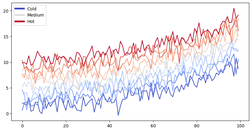
DataFrames
import pandas as pd
import numpy as np
df = pd.DataFrame(
    {
        "A": 1.0,
        "B": pd.Timestamp("20130102"),
        "C": pd.Series(1, index=list(range(4)), dtype="float32"),
        "D": np.array([3] * 4, dtype="int32"),
        "E": pd.Categorical(["test", "train", "test", "train"]),
        "F": "foo",
    }
)
df.head()
C:\Users\Pawel.kaminski\AppData\Local\Temp\ipykernel_21596\386600454.py:1: DeprecationWarning:
Pyarrow will become a required dependency of pandas in the next major release of pandas (pandas 3.0),
(to allow more performant data types, such as the Arrow string type, and better interoperability with other libraries)
but was not found to be installed on your system.
If this would cause problems for you,
please provide us feedback at https://github.com/pandas-dev/pandas/issues/54466
import pandas as pd
Multimedia
To add images, videos, etc. to your interactive notebook, use the display tools from the IPython library. See the official documentation for all the objects you can use and their configuration. Please find examples of adding multimedia to your book below.
Images
from IPython.display import Image
Image("./assets/common/uni_logo.png")
Videos
from IPython.display import Video
Video("./assets/05_ipynb_guidelines/vid-sample.mp4")YouTube/Vimeo videos
Dedicated IPython.display tools make adding an embedded video hosted on YouTube or Vimeo very easy. You just have to find an ID of the video you want to use and write it inside brackets and quotation marks, e.g. for ID 266248400 you can construct the VimeoVideo("266248400") object.
Finding a video’s ID is usually more tricky.
In YouTube, the video’s ID is in the link of the video between ?v= and & characters. For example, for a link "https://www.youtube.com/watch?v=D-IG-Skh8p8&pp=ygUKZGUgZ3J1eXRlcg%3D%3D" the ID is D-IG-Skh8p8.
from IPython.display import YouTubeVideo
YouTubeVideo("D-IG-Skh8p8")It is simpler in Vimeo. The ID is just the part of the URL right after the last / slash. For example, in the link to "https://vimeo.com/266248400" the ID is the 266248400.
from IPython.display import VimeoVideo
VimeoVideo("266248400")Please note that the placement of the video’s ID can be changed by either YouTube or Vimeo.
Markdown
Input:
#### Heading 4

With some exceptions, the MyST markdown rules apply.

1. First item
2. Second item
    * First sub-item

| Header 1     | Header 2     |
| :---         | ---:         |
| Row 1, Col 1 | Row 1, Col 2 |


```{note}
Even directives like admonitions are to some extent supported.
```
Output:
Heading 4
With some exceptions, the MyST markdown rules apply.
First item
Second item
First sub-item
| Header 1 | Header 2 |
|---|---|
| Row 1, Col 1 | Row 1, Col 2 |
Math
We recommend using the dollar-sign syntax or the {math} directive for writing mathematical expressions.
Dollar-sign syntax
Input:
$$\left( \sum_{k=1}^n a_k b_k \right)^2 \leq \left( \sum_{k=1}^n a_k^2 \right) \left( \sum_{k=1}^n b_k^2 \right)$$
Output:
{math} directive
Input:
\left( \sum_{k=1}^n a_k b_k \right)^2 \leq \left( \sum_{k=1}^n a_k^2 \right) \left( \sum_{k=1}^n b_k^2 \right)
Output:
LaTeX syntax (not supported)
LaTeX syntax without the {math} directive will not work, even if it renders correctly in Jupyter Notebook or Jupyter Lab. Take for example the same equation but written in pure LaTeX syntax:
Input:
\begin{equation*}
\left( \sum_{k=1}^n a_k b_k \right)^2 \leq \left( \sum_{k=1}^n a_k^2 \right) \left( \sum_{k=1}^n b_k^2 \right)
\end{equation*}
Output:
Formatting output of your code
The formatting of code outputs is highly configurable. Please find examples of how to format particular outputs and even insert outputs into other locations of the document in the official documentation.
Many libraries support their own HTML output formatting, and this generally carries over to Jupyter Book outputs as well. For example, the following cell uses Pandas to format cells based on their values:
import numpy as np
import pandas as pd

np.random.seed(24)
df = pd.DataFrame({'A': np.linspace(1, 10, 10)})
df = pd.concat([df, pd.DataFrame(np.random.randn(10, 4), columns=list('BCDE'))],
               axis=1)
df.iloc[3, 3] = np.nan
df.iloc[0, 2] = np.nan

def color_negative_red(val):
    """
    Takes a scalar and returns a string with
    the css property `'color: red'` for negative
    strings, black otherwise.
    """
    color = 'red' if val < 0 else 'black'
    return 'color: %s' % color

def highlight_max(s):
    '''
    highlight the maximum in a Series yellow.
    '''
    is_max = s == s.max()
    return ['background-color: yellow' if v else '' for v in is_max]

df.style.\
    applymap(color_negative_red).\
    apply(highlight_max).\
    set_table_attributes('style="font-size: 10px"')
C:\Users\Pawel.kaminski\AppData\Local\Temp\ipykernel_21596\2549200461.py:28: FutureWarning: Styler.applymap has been deprecated. Use Styler.map instead.
applymap(color_negative_red).\
See the Pandas Styling docs for more information about styling DataFrames, and check out the documentation of your library of choice to see if they support similar features.
Adding interactivity
Jupyter Notebook has support for many kinds of interactive outputs, including the ipywidgets ecosystem as well as many interactive visualization libraries. These are supported in Jupyter Book, with the right configuration. This page has a few common examples.
First off, we’ll download a little bit of data and show its structure:
import plotly.express as px
data = px.data.iris()
data.head()import altair as alt
alt.Chart(data=data).mark_point().encode(
x="sepal_width",
y="sepal_length",
color="species",
size='sepal_length'
)from bokeh.plotting import figure, show, output_notebook
output_notebook()
p = figure()
p.circle(data["sepal_width"], data["sepal_length"], fill_color=data["species"], size=data["sepal_length"])
show(p)