General Remarks and Limitations
All dynamic functionalities must be performed in a browser of anyone who views your book. This is a very powerful solution but has its limitations. Some dynamic features require a server or a database, which are not provided in our setup. If a feature cannot be performed in a viewer’s browser, it will not be rendered in your digital book and can even break part of your book of being shown.
Nearly all dynamic functionalities that can be shown in a static web page can be included in a digital version of your book as well. This includes interactive maps, graphs, charts, diagrams, animations, video or audio players, and even games your readers can play – as long as it doesn’t require a running server.
Figure 4.1: Tic tac toe game working without a server. License: MIT.
“Will I Be Able To Use My Pre-Existing Jupyter Notebook?”
Yes, you will be able to use your pre-existing Jupyter notebook. We can show your Jupyter notebook (data, code and outputs), but we will not execute your code for you. You must execute your notebook and export its outputs in a way described in the next chapter. This solution gives you great flexibility in generating your book’s contents. This means that you should be able to use the work you have done on your .ipynb file, regardless which Python version you have been using (or maybe you used something completely different instead), what are the libraries that you have chosen, what hardware you operated on (for example you can perform your computations utilizing GPU instead of CPU), etc. It should work as expected, assuming the generated output can be included in a static web page.
Thinking About Longevity
When preparing your book for publishing, please consider its life after the release. Whenever you include a link to an external source, bear in mind that a target of such link might change or cease to exist in the future.
You should also apply this caution when dealing with any other external sources. Whenever you directly or indirectly use a resource that is hosted by a service like YouTube, Vimeo, Sketchfab, Observable, GitHub, Google Drive, Google Sheets, Tableau, etc., you have to take note of its terms of service. In general, there is no guarantee that a source hosted there will stay unchanged. Wherever possible, include files directly in your assets folder instead of links to resources.
Non-Dynamic Objects
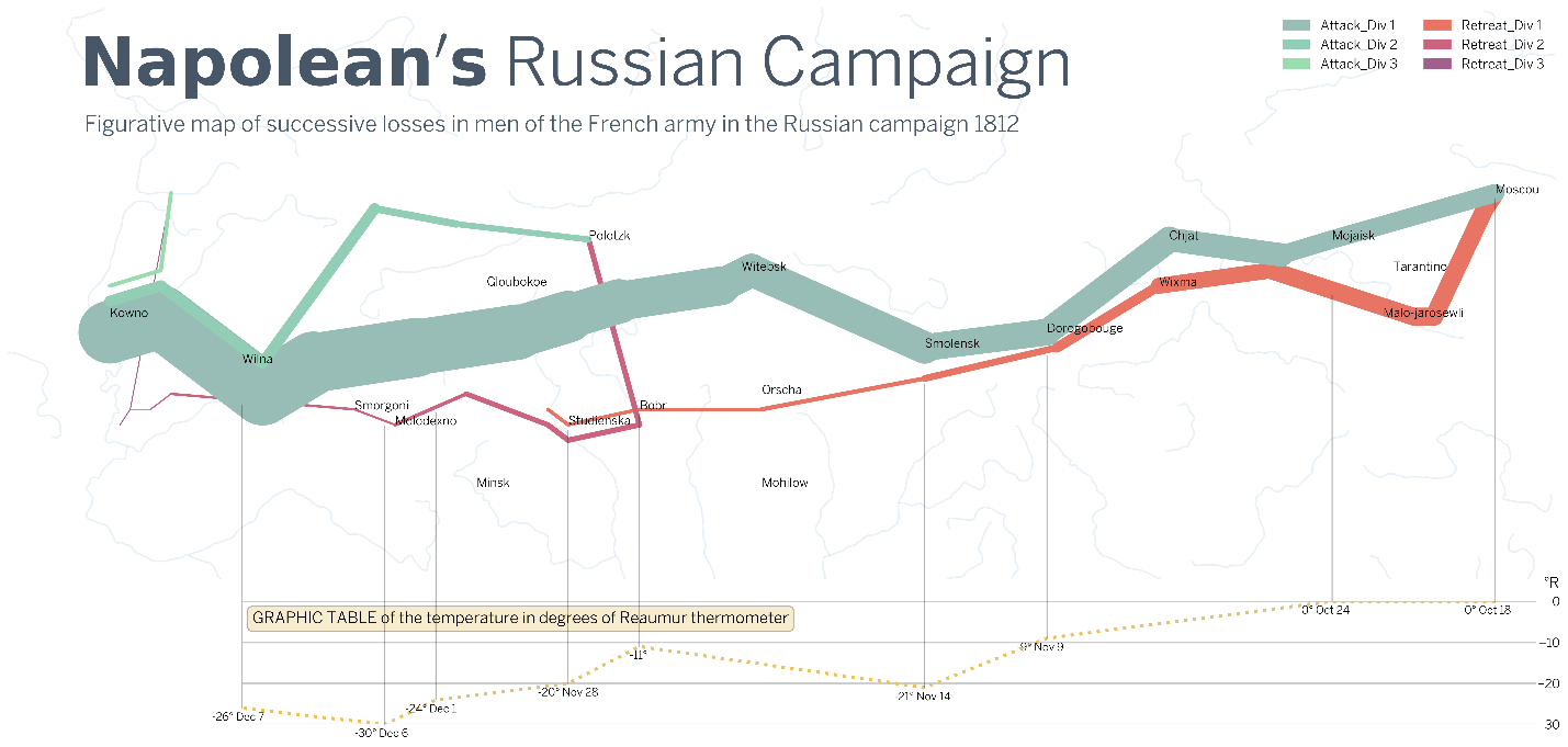
Say you already have a Jupyter notebook, but instead of incorporating it as a whole in your book you want to include a single visualization generated in it. As an example, let take a the famous Charles Minard’s chart recreated by Amit Amola using Python and Matplotlib. The process of exporting it as an image is very simple, but it depends on which notebook application you are using.
Figure 4.2: Recreation of Minard’s Chart of Napoleon’s Russian Campaign made by Amit Amola (GPL-3.0 license).
Jupyter Notebook / Google Colab
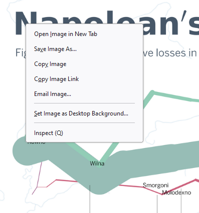
In Jupyter Notebook or in Google Colab, just right click on a visualization, save the image and import it in your .docx file as you normally would with an image.
Figure 4.3: Saving object from Jupyter Notebook as an image. Example map made by Amit Amola (GPL-3.0 license).
Jupyter Lab
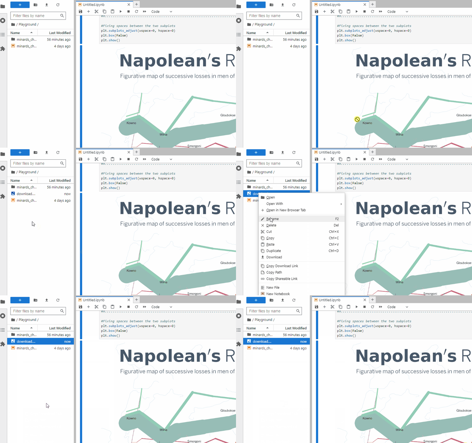
In Jupyter Lab, you can just drag-and-drop the output of your notebook to the File Browser tab on the left of the screen. Download the object and insert it in your .docx file as you normally would with an image.
Figure 4.4: Saving object from Jupyter Lab as an image. Example map made by Amit Amola (GPL-3.0 license).
Objects Inside Your Word Processor
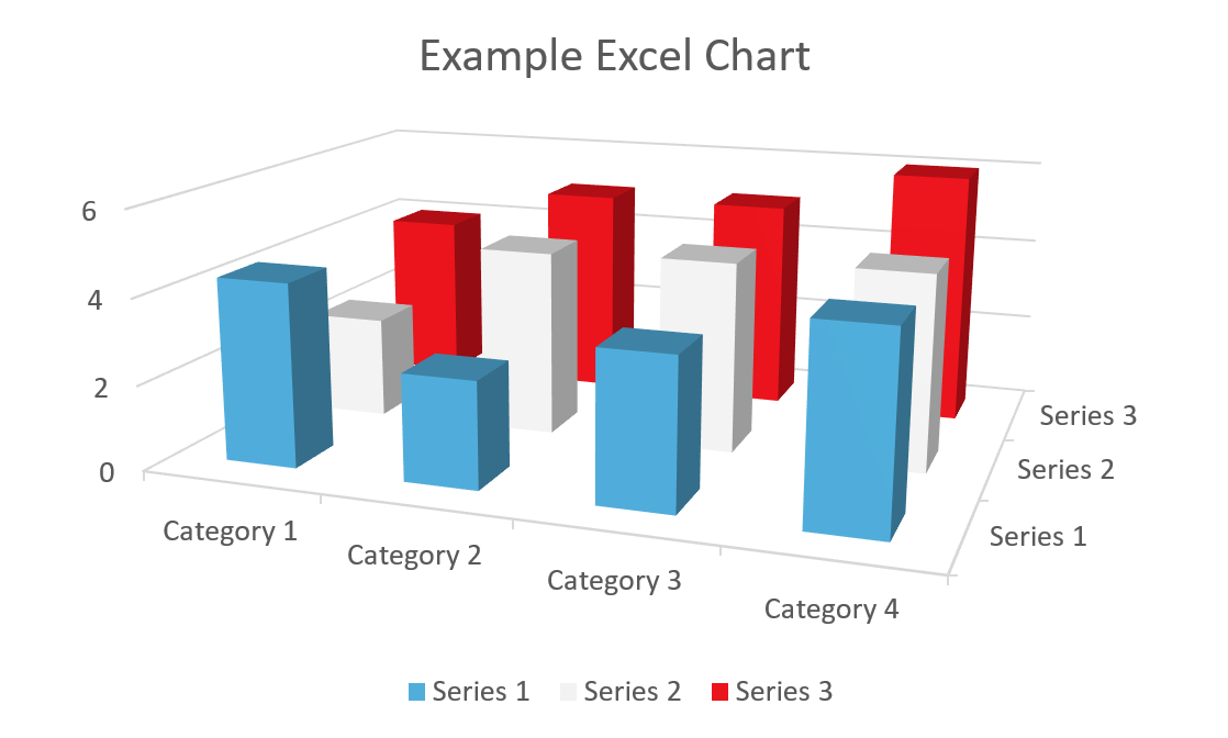
You can also enrich your book with objects from your MS Word, MS Excel, MS PowerPoint, etc. This includes, among others, Charts, 3D models, WordArts and SmartArts objects. However, just inserting them to your .docx file will not work. Instead, you must save them to a separate file and reference them in your metadata table, at least in the “## Original” field. It is recommended that you take a screenshot of your object and use the image as the “## Digital input” and the “## Paper input” in the metadata table as well. Bear in mind that such screenshots are required to have high quality to be published.
Figure 4.5: Example of a metadata table referencing an Excel chart.

Figure 4.6: Excel chart rendered from the metadata table.
Sketchfab 3D Models
You can easily include a 3D model hosted on Sketchfab in your book. To do that go to the web page on sketchfab.com, select the “Embed” option and copy to clipboard the code (including the embed wrapper div). Save this div in a html file in your book’s assets directory. Then use metadata table and the “## Digital input” field to point to the new html file. Please be aware that using this method your book only references a 3D model. If it is removed from Sketchfab or moved to a different place, your book will point to an empty location.
Figure 4.7: Kinora 3D model by Tim van der Heijden (license CC-BY-4.0).
Dynamic JavaScript Objects
JavaScript is a language that was specifically designed to run natively in web browsers. This means that all modern web browsers can interpret and run JavaScript code without needing any additional plugins or tools. On the other hand, tools like Jupyter Notebooks are fantastic tools for data analysis and exploration, but they’re not designed for creating elements of interactive web pages.
Using Observable Notebook
The easiest way to include a JavaScript object, like a map or a graph, is to use the export option of an Observable notebook.
For example, if you would like to include this chart in your book, here are the steps to follow.
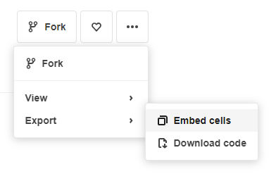
Step 1
Figure 4.8: Click on the “Embed cells” button.
Step 2
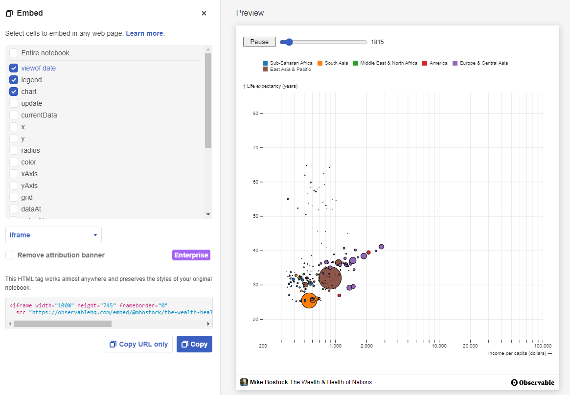
Figure 4.9: Select cells to embed, click “Copy URL only”.
Step 3
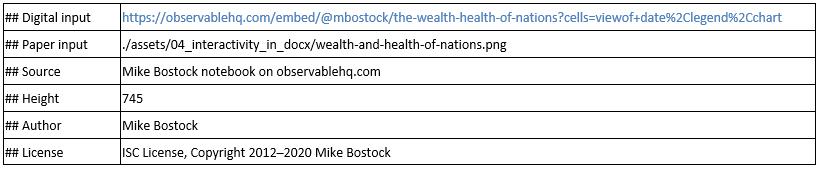
Figure 4.10: In your Word file, create a Metadata table. Make sure it has a a) “##Digital input” field with the URL you’ve copied from the Observable notebook and b) “##Height” field with “height” value from the <iframe> snippet shown at the bottom of the page in Observable. Remember to add appropriate metadata about the author and the source.
Result
Figure 4.11: Income per capita, population and life expectancy 1800-2005 graph made by Mike Bostock and published under ISC License.
This method should work on almost every visualization as long as the Observable portal supports exporting objects as <iframe>. Some other examples are available here. Please note that when you embedded external source in your manuscript, your book depends on this source. Keep it in mind when thinking about longevity of your work.
Other JavaScript Objects
If you feel competent in your skills in programming JavaScript, you can try to write your own html file and embed it in your book. This might be an interesting solution to include a custom JavaScript widget or visualization in your book. To embed a custom html file in your book, write the html location as the “##Digital input” in a metadata table.
Figure 4.12: Locations around the World of University of Luxembourg and De Gruyter.
A common use case for embedding html inside of a book are zoomable images.
Figure 4.13: Example of a zoomable image. Source: Dario Morelli, 2012.
AI-generated content may be incorrect." width=“100%”>
Writing code for maps, graphs, diagrams, etc. is a skill on its own. Please refer to separate documentation appropriate for a given topic to have a better understanding of how to construct such elements.
Another challenge is to get and transform data to use in your visualization. Here is an example of fetching a TopoJSON data before constructing a map.
Figure 4.14: Map of Poland as of April 1938 made by Iwona Rajca, @EveTheAnalyst. See also a tutorial on making similar maps.
Our platform for digital publishing gives you great flexibility regarding the elements you can embed in your book. Nearly every object that can be embedded as a <iframe> html object can be also part of your book. Use this ability with highest responsibility.
Dynamic Objects From Jupyter Notebook
Jupyter Widgets
There is a subset of Jupyter interactive visualizations called jupyter-widgets that do not need a server to add interactivity to your book called.
Step 1
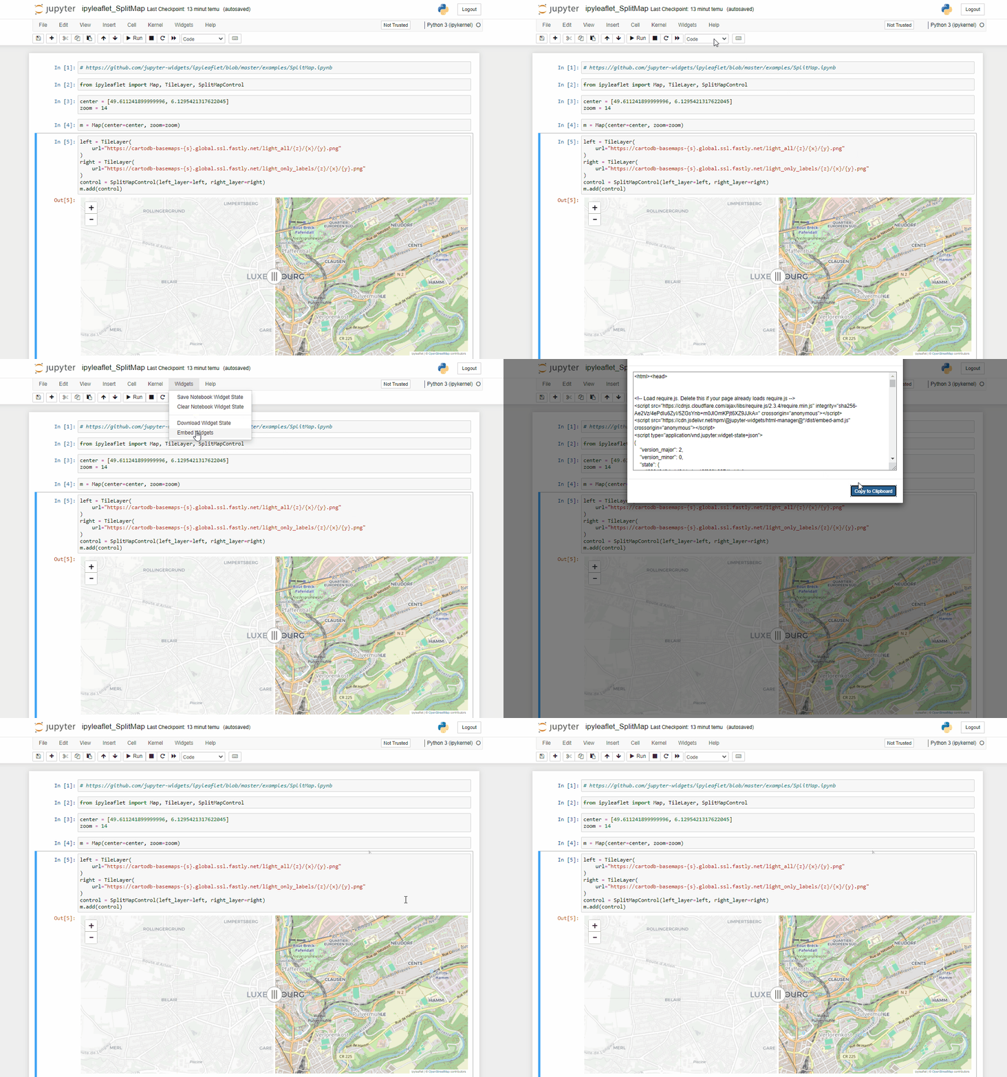
Copy the html object (in Jupyter notebook select “Widgets” > “Embed Widgets” > “Copy to Clipboard”).
Figure 4.15: Example of accessing html describing a map in Jupyter Notebook.
Step 2
Paste the copied data into .html file.
Step 3
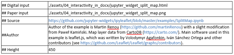
Point to .html file in your .docx file.
Figure 4.16: Example of Metadata Table to insert html to your manuscript.
Result
Jupyter Notebooks As HTML
You can also include the whole .ipynb notebook inside an .docx file. To do that, just export the contents of your .ipynb to .html and refer to this .html file in a metadata table. How to perform the export operation depends on the tool you are using.
In Jupyter notebook, you must click the “File” button in the top left corner of the window and select “Download as” > “HTML (.html)”.
In Jupyter Lab, select “File” > “Save and Export Notebook As…” > “HTML”.
Then just reference the .html file in the metadata table in your .docx file.


Figure 4.17: Monthly distribution of passengers (1949-1960).
If interactivity works in the stand-alone .html file, it most likely will also work in the digital version of your book.
JupyterLite
Feature to be added in future releases.
To give your readers availability to interact with your code, one option is to use the JupyterLite. Because it runs entirely in the browser and does not need a server, you will be able to include it a digital version of your book.
To include a JupyterLite terminal inside your digital page, insert a metadata table referring to the JupyterLite demo hosted on GitHub. You can also choose among available options, e.g. Jupyter Lab vs Jupyter Notebook, Python vs JavaScript, etc. In this example, we do not point to any “## Paper input”, so that our paper version will leave that object out entirely.
Python example
Here is an exemplary code you can try:
from sklearn import datasets
import matplotlib.pyplot as plt

iris = datasets.load_iris()
_, ax = plt.subplots()
scatter = ax.scatter(iris.data[:, 0], iris.data[:, 1], c=iris.target)
ax.set(xlabel=iris.feature_names[0], ylabel=iris.feature_names[1])
_ = ax.legend(
 scatter.legend_elements()[0], iris.target_names, loc="lower right", title="Classes"
)
JavaScript example